Journal Club: GraftM, a tool for scalable, phylogenetically informed classification of genes within metagenomes

A paper recently caught my eye for two reasons: (1) it implemented an idea that someone smart recently brought up to me and (2) it perfectly illustrates the question of "functional resolution" that comes up in the functional analysis of metagenomes.

The paper is called GraftM: a tool for scalable, phylogenetically informed classification of genes within metagenomes, by Joel A. Boyd, Ben J. Woodcroft and GeneW. Tyson, published in Nucleic Acids Research.

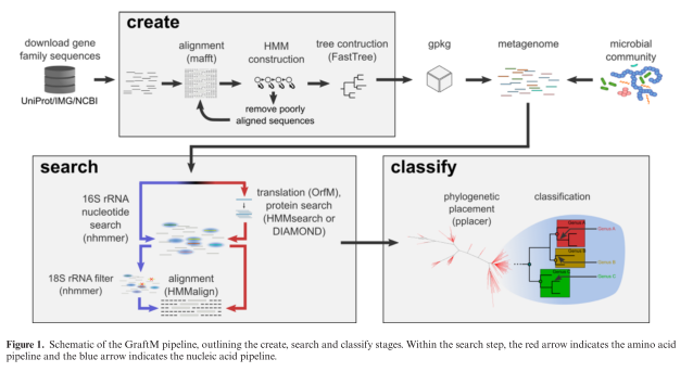
The tool that they present is called GraftM, and it does something very clever (in my opinion). It analyzes DNA sequences from mixtures of microbes (so-called "metagenomes" or microbiome samples) and it identifies the allele of a collection of genes that is present. This is a nice extrapolation of the 16S classification process to include protein-coding sequences, and they even use the software package pplacer, which was developed for this purpose by Erick Matsen (Fred Hutch). Here's their diagram of the process:

They present some nice validation data suggesting that their method works well, which I won't reproduce here except to say that I'm always happy when people present controls. 

Now instead of actually diving into the paper, I'm going to ruminate on the concept that this approach raises for the field of functional metagenomics.

Functional Analysis

When we study a collection of microbes, the "functional" approach to analysis considers the actual physical functions that are predicted to be carried out by those microbes. Practically, this means identifying sets of genes that are annotated with one function or another using a database like KEGG or GO. One way to add a level of specificity to functional analysis is to overlay taxonomic information with these measurements. In other words, not only is Function X encoded by this community, we can say that Function X is encoded by Organism Y in this community (while in another community Function X may be encoded by Organism Z). This combination of functional and taxonomic data is output by the popular software package HUMAnN2, for example. 

Let's take a step back. I originally told you that protein functions were important (e.g. KEGG or GO labels), and now I'm telling you that protein functions ~ organism taxonomy is important. The difference is one of "functional specificity."

Functional Specificity

At the physical level, microbial communities consist of cells with DNA encoding RNA and producing proteins, with those RNA and protein molecules doing some interesting biology. When we summarize those communities according to the taxa (e.g. species) or functions (e.g. KEGG) that are present, we are taking a bird's eye view of the complexity of the sample. Adding the overlay of taxonomy ~ function (e.g. HUMAnN2) increases the specificity of our analysis considerably.

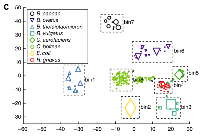
Now take a look at the figure above. You can see that a single KEGG group actually consists of a whole family of protein sequences which have their own phylogenetic relationships and evolutionary history. This tool (GraftM) presents a means of increasing the level of functional resolution to differentiate between different protein sequences (alleles) that are contained within a single functional grouping (e.g. KEGG label). However, it should be noted that this approach is much more computationally costly than something like HUMAnN2, and is best run on only a handful of protein families at a time. 

Summary

Lastly, let me say that there is no reason why a higher or lower level of functional specificity is better or worse. There are advantages at both ends of the spectrum, for computational and analytical reasons that would be tiresome to go into here. Rather, the level of functional specificity should be appropriate to the biological effect that you are studying. Of course, it's impossible to know exactly what will be the best approach a priori, which is why it's great to have a whole collection of tools at your disposal to test your hypothesis in different ways. 

Detecting viruses from short-read metagenomic data

My very first foray into the microbiome was in graduate school when my advisor (Dr. Rick Bushman) suggested that I try to use a high-throughput genome sequencing instrument (a 454 pyrosequencer) to characterize the viruses present in the healthy human gut. That project ended up delving deeply into the molecular evolution of bacteriophage populations, and gave me a deep appreciation for the unpredictable complexity of viral genomes. 

While I wasn't the first to publish in this area, the general approach has become more popular over the last decade and a number of different groups have put their own spin on it. 

Because of the diversity of viruses, you can always customize and enhance different aspects of the process, from sample collection, purification, and DNA isolation to metagenomic sequencing, bioinformatic analysis, and visualization. It's been very interesting to see how sophisiticated some of these methods have become.

On the bioinformatic analysis side of things, I ended up having the most success in those days by assembling each viral genome from scratch and measuring the evolution of that genome over time. More of the bespoke approach to bioinformatics, rather than the assembly line. 

In contrast, these days I am much more interested in computational approaches that allow me to analyze very large numbers of samples with a minimum of human input required. For that reason I don't find de novo assembly to be all that appealing. It's not that the computation can't be done, it's more than I have a hard time imagining how to wrap my brain around the results in a productive way. 

In contrast, one approach that I have been quite happy with is also much more simple minded. Instead of trying to assemble all of the new genomes in a sample, it's much easier to simply align your short reads against a reference database of viral genomes. One of the drawbacks is that you can only detect a virus that has been detected before. On the other hand, one of the advantages is also that you can only detect a virus that has been detected before, meaning that all samples can be rapidly and intuitively compared against each other. 

To account for the rapid evolution of viral genomes, I think it's best to do this alignment in protein space against the set of proteins contained in every viral genome. This makes the alignments a bit more robust. 

If you would like to perform this simple read alignment method for viral detection, you can use the code that I've put together at this GitHub repo. There is also a Quay repository hosting a Docker image that you can use to run this analysis without having to install any dependencies. 

This codebase is under active development (version 0.1 at time of writing) so please be sure to test carefully against your controls to make sure everything is behaving well. At some point I may end up publishing more about this method, but it may be just too simple to entice any journal. 

Lastly, I want to point out that straightforward alignment of reads does not account for any number of confounding factors, including but not limited to:

1. presence of human or host DNA
2. shared genome segments between extant viruses
3. novel viral genomes
4. complex viral quasi-species
5. integration of prophages into host genomes

There are a handful of tools out there that do try to deal with some of those problems in different ways, quite likely to good effect. However, it's good to remember that with every additional optimization you add a potential confounding factor. For example, it sounds like a good idea to remove human sequences from your sample, but that runs the risk of also eliminating viral sequences that happen to be found with the human genome, such as lab contaminants or integrated viral genome fragments. There are even a few human genes with deep homology to existing viral genes, thought to be due to an ancient integration and subsequent repurposing. All I mean to say here is that sometimes it's better to remove the assumptions from your code, and instead include a good set of controls to your experiment that can be used to robustly eliminate signal coming from, for example, the human genome. 

Journal Club: Discovering new antibiotics with SLAY

This paper is a bit of a departure for me, but even though it's not a microbiome paper it's still one of the most surprising and wonderful papers that I've seen in the last year, so bear with me.

We're looking at Tucker, et al. "Discovery of Next-Generation Antimicrobials through Bacterial Self-Screening of Surface- Displayed Peptide Libraries" Cell 172:3, 2018. (http://www.cell.com/cell/fulltext/S0092-8674(17)31451-4).

When I first learned about this project, I said, "That's a fun idea, but it won't possibly work," to which the PI responded, "We've already done it." 

The extremely cool idea here was to rapidly discover new antibiotics by quickly screening an immense library of novel peptides. The diagram below lays it out: they created a library of peptides, expressed those peptides on the surface of E. coli, and then used genome sequencing to figure out which of those peptides were killing the bacteria. The overall method is called SLAY, which exceedingly clever.

While this idea seems simple, there are more than a few parts that I thought would be impossibly difficult. They include (a) building a sufficiently large library of peptides, (b) expressing those peptides on the surface of the bacteria and not inside the cell, and (c) making sure that the peptides were only killing the cells they were tethered to and not any neighbors. 

I won't go through the entire paper, but I will say that the authors ended up doing quite a bit of work to convince the readers that they actually discovered new antimicrobial peptides, and that they weren't observing some artifact. At the end of the day it seems pretty irrefutable to me that they were able to use this entirely novel approach in order to identify a few new antibiotic candidates, which typically takes hundreds of millions of dollars and decades of work. 

In short, it looks like smart people are doing good work, even outside of the microbiome field. I'll definitely be keeping an eye on these authors to see what they come up with next!

Journal Club: Metagenomic binning and association of plasmids with bacterial host genomes using DNA methylation

Amid the holiday rush last month, I was gratified to see a publication describing a new computational method that had been on my mind. 

The paper is "Metagenomic binning and association of plasmids with bacterial host genomes using DNA methylation", published in Nature Biotechnology on December 11, 2017. 

The Concept

Bacteria do something funny to their DNA that you may not have heard of. It's called covalent DNA modification, and it often consists of adding a small methyl group to the DNA molecule itself. This added methyl group (or hydroxyl, or hydroxymethyl, etc.) doesn't interfere with the normal operation of DNA (making RNA, and more DNA). Instead it serves as a marker that differentiates self-DNA from invading DNA (such as from a phage, plasmid, etc.).

For example, one species may methylate the motif ACCGAG (at the bolded base), while another might methylate CTGCAG. If the first species encounters a ACCGAG motif that lacks the appropriate methyl, it treats it as invading DNA and chews it up.

The ongoing arms race of mobile DNA elements has helped maintain a diversity of DNA modifications, such that many different species of bacteria have a unique profile. 

The interesting trick here is that we now have a way to read out the methylation patterns in DNA in addition to the sequence. This is most notably available via PacBio sequencing, which typically will generate a smaller number of much longer sequence fragments than other genome sequencing methods. Bringing it all together, the authors of this paper were able to use the methylation patterns from PacBio sequencing to much more accurately reconstruct the microbes present in a set of environmental samples (such as the human microbiome). 

The Data

The approach of the authors was to first assemble the PacBio sequences, and then bin those larger genome fragments together based on a common epigenetic signature. 

Figure 2c shows the binning of genome fragments in a sample containing a known mixture of bacteria.

Figure 2e shows the binning of genome fragments in a gut microbiome sample containing a mixture of unknown bacteria (and viruses, fungi, etc.).

In general, this seems like a very interesting approach. After my read of the paper, it appears that the bacteria present in the microbiome contain a distinct enough set of epigenetic patterns to enable the deconvolution of many different species and strains. I look forward to seeing how this method stacks up against other binning approaches in the future. 

Final note

For those of you interested in phage and mobile genetic elements, I wanted to point out that the authors also explore a topic that has been studied somewhat by others – the linkage of phage to their hosts via epigenetic signatures. The idea here is that it can be computationally difficult to match a phage genome or plasmid with its host. One experimental method that accomplishes this is Hi-C, which takes advantage of the physical proximity of the host genome within an intact cell. In contrast, the PacBio method does not require intact cells, and can be used to link phage or plasmids with their host based on a shared epigenetic signature. 

My hope is that this type of data starts to become more widely available. There are clearly a number of computational tools that need to be refined in order to get full use of all this information, but it does seem to hold a good deal of promise. 

Journal Club: A role for bacterial urease in gut dysbiosis and Crohn’s disease

It's nice when you see a new paper describing the type of science that you find the most exciting and relevant, and doubly so when it's written by a group of people that you know and respect. Full disclosure: this paper is from the group that I did my graduate work with at the University of Pennsylvania, and there's quite a lot to talk about. 

Ni, J. et al. (2017) ‘A role for bacterial urease in gut dysbiosis and Crohn’s disease’, Science Translational Medicine, 9(416), p. eaah6888. doi: 10.1126/scitranslmed.aah6888.

Building a model for microbiome research

Before talking about what the authors did, I want to describe how they did it. They started (in a previous study) with a cohort of patients being treated for a common disease with no known cure (Crohn's) and looked for differences in the genomic content of their microbiome compared to healthy control subjects. That initial analysis indicated that one particular metabolic pathway was enriched in patients with the disease. In this study they followed up on that finding by analyzing the metabolites produced by those microbes. The combination of those two orthogonal analyses (genomic DNA and fecal metabolites) provided some suggestion that microbes in the gut were producing one particular chemical which may have a role in disease. To test that hypothesis they moved into a mouse model where they could test that hypothesis with controlled experiments, not only adding and removing microbes but also tracking the passage of metabolites via isotopic labelling. That model system provided crucial data that supported the findings from the human clinical samples – that a specific bacterial enzyme may have a role in human disease. After this study, I can only imagine that the next step would be to move back into humans and see if that target can be used to generate a useful therapeutic. 

The microbiome field is relatively new, and I believe that its first batch of groundbreaking therapeutics is just over the horizon. I wouldn't be surprised if the most influential studies in this field follow a trajectory that is similar to what I describe above: generating hypotheses in humans, testing them in animal models, and moving back to human to test and deliver therapeutics. 

Ok, enough predictions, let's get into the paper.

The Microbiome – Who's Who and What's What

Fig. 2. Associations between bacterial taxa abundance ascertained by fecal shotgun metagenomic sequencing and the fecal metabolome in healthy pediatric subjects and those with Crohn’s disease.

The figure above shows the association between Who's in the microbiome (bacterial genera, vertical axis) and What's (metabolites, horizontal axis) in the microbiome. The point here is that certain microbes are associated with certain metabolites, with a big focus on the amino acids that are being produced. The prior set of experiments suggested that the microbes in Crohn's patients had an increased capacity for producing amino acids, while this figure (and Figure 1) goes further to show that there is a subset of microbes associated with higher actual levels of amino acids in those subjects.

Tracking metabolism in the microbiome

Here's a deceptively simple figure describing a powerful finding. 

Fig. 3. In vivo heavy isotope assays using 15N-labeled urea to determine the effect of bacterial urease on nitrogen flux in the murine gut microbiota.

This experiment uses radiolabelled urea to measure the production of lysine by microbes in the gut. The central question here is what is producing the extra amino acids in Crohn's disease? In this experiment the authors added radiolabelled urea so that they could track how much lysine was being produced from that urea. Crucially, they found that adding either antibiotics or a defined set of microbes (called "ASF") reduced the amount of lysine that was produced from that urea, which supports the hypothesis that microbes in the gut are directly metabolizing urea. 

Tying it all together

Fig. 6. Effect of E. coli urease on colitis in a T cell adoptive transfer mouse model of colitis

I've skipped over a lot of interesting control experiments so that I could get to the grand finale. Everything I've told you up until now has established that (a) Crohn's patients have higher levels of certain amino acids in their stool, (b) those high amino acid levels are associated with particular bacteria, and (c) bacteria in the gut are able to produce amino acids from urea. To bring it all together the authors went to a mouse model of colitis to see whether adding or removing a single gene would have an effect on disease. They found that E. coli with urease (an enzyme that metabolizes urea) caused significantly more disease than E. coli without urease. This brings it all back to the action of a single gene on a model of human disease, which is the classic goal of reductionist molecular biology, but the gene of interest is encoded by the human microbiome. 

I think that's pretty cool. 

From here it's easy to imagine that people might be interested in designing a drug that targets microbial urease in order to reduce human disease, although that's got to be a pretty difficult task and I have no idea how diverse bacterial urease enzymes are. 

Bringing it back to my first point, this seems like the best case example of how to advance our understanding of the human microbiome with the goal of treating human disease. I hope to see many more like it in the years to come.

Making sparse DataFrames efficiently

Here's a little story about a computational challenge that I came across recently, and how a little bit of performance profiling went a long way to improve my analysis.

Background

I've been working with a large amount of data recently, and my principal bottleneck hasn't been the raw sequence analysis, but rather analyzing the results across large numbers of samples. For context, I'm working with thousands of samples, each of which contains 10,000 - 10,000,000 observations. The raw data was terabytes of raw genomic sequence data, and so I'm definitely working with a more compact data structure, but it's still quite a bit of data to work with in memory. 

There have been a few different iterations for this workflow, starting by working in memory (started swapping), then moving to a PostgreSQL database (which was too slow with read/write), and now working in memory on a larger machine using sparse matrices (following a helpful suggestion from Jonathan Golob).

What I've really liked about these sparse matrices is that it's incredibly fast to slice the data in different ways, which is what I need to be able to figure out both (a) how similar samples are to each other and (b) how different observations are distributed across samples. In other words, I need to be able to retrieve the data quickly in a column-wise or row-wise manner and sparse matrices really help with this.  Also, my underlying data is very sparse, which is to say that a vast majority of the cells in my table are 0 or N/A. Lastly, they're supported in Pandas, which is really great. 

The Challenge

While it's really quick to query these sparse matrices, I've been finding it difficult to make them. This morning I did a bit of performance profiling to compare a few different ways of constructing these tables and I found that not all construction methods are created equal. You can find my profiling code here, if you're interested (this was run in Pandas 0.20.3). 

The data that I'm working with is a set of observations that are originally constructed in longitudinal format, with every observation as an item in a list that includes the row name, column name, and cell value. What I wanted to see was what the most efficient method would be to make this into a sparse table in wide format, which could be indexed and sliced easily by row or column. 

Options

1. Sparse DataFrame from nested dictionaries: Make a nested dictionary with the first level of keys as column labels and the second level of keys as row labels, and then convert directly to the SparseDataFrame.

2. Column-wise addition to sparse DataFrame: Make an empty SparseDataFrame and then sequentially add in the data from each column. 

3. Dense longitudinal, pivot, then make sparse: Make a dense DataFrame from the longitudinal data, pivot it in dense format, and then make it into a SparseDataFrame.

4. Sparse longitudinal DataFrame, then pivot: Make a SparseDataFrame in longitudinal format and then pivot it in to wide format. 

Results

I tested each of the above options using four different matrices of varying sizes:

Matrix: 60 rows, 67 cols, 2.463% full

1. Testing sparse DataFrame from nested dictionaries
29.6 ms ± 2.33 ms per loop (mean ± std. dev. of 7 runs, 10 loops each)

2. Testing columnwise addition to sparse DataFrame
41.5 ms ± 813 µs per loop (mean ± std. dev. of 7 runs, 10 loops each)

3. Testing make dense DataFrame from longitudinal format, pivot it, then convert to sparse
33.1 ms ± 1.07 ms per loop (mean ± std. dev. of 7 runs, 10 loops each)

4. Testing make sparse DataFrame from longitudinal format, then pivot it
19 ms ± 1.39 ms per loop (mean ± std. dev. of 7 runs, 100 loops each)


Matrix: 100 rows, 100 cols, 9.54% full

1. Testing sparse DataFrame from nested dictionaries
61.2 ms ± 8.28 ms per loop (mean ± std. dev. of 7 runs, 10 loops each)

2. Testing columnwise addition to sparse DataFrame
97.7 ms ± 15 ms per loop (mean ± std. dev. of 7 runs, 10 loops each)

3. Testing make dense DataFrame from longitudinal format, pivot it, then convert to sparse
57.3 ms ± 2.15 ms per loop (mean ± std. dev. of 7 runs, 10 loops each)

4. Testing make sparse DataFrame from longitudinal format, then pivot it
101 ms ± 4.46 ms per loop (mean ± std. dev. of 7 runs, 10 loops each)


Matrix: 100 rows, 632 cols, 1.574% full

1. Testing sparse DataFrame from nested dictionaries
1.29 s ± 50.7 ms per loop (mean ± std. dev. of 7 runs, 1 loop each)

2. Testing columnwise addition to sparse DataFrame
1.41 s ± 40.4 ms per loop (mean ± std. dev. of 7 runs, 1 loop each)

3. Testing make dense DataFrame from longitudinal format, pivot it, then convert to sparse
1.19 s ± 13.6 ms per loop (mean ± std. dev. of 7 runs, 1 loop each)

4. Testing make sparse DataFrame from longitudinal format, then pivot it
94 ms ± 1.07 ms per loop (mean ± std. dev. of 7 runs, 10 loops each)


Matrix: 100 rows, 1000 cols, 9.526% full

1. Testing sparse DataFrame from nested dictionaries
2.82 s ± 29.1 ms per loop (mean ± std. dev. of 7 runs, 1 loop each)

2. Testing columnwise addition to sparse DataFrame
3.15 s ± 81.9 ms per loop (mean ± std. dev. of 7 runs, 1 loop each)

3. Testing make dense DataFrame from longitudinal format, pivot it, then convert to sparse
2.8 s ± 72.5 ms per loop (mean ± std. dev. of 7 runs, 1 loop each)

4. Testing make sparse DataFrame from longitudinal format, then pivot it
826 ms ± 30.8 ms per loop (mean ± std. dev. of 7 runs, 1 loop each)

Summary

In the results above you can see that in general the fastest method was #4 – making the DataFrame sparse in longitudinal format, and then pivoting it into wide matrix format. However, I need to stress that the relative performance of each of these methods varied widely depending on how sparse the matrix was. In general, option #4 worked better with sparser datasets, but I haven't fully tested the range of parameter space varying the number of rows, columns, and values. 

A larger point that I could also make here is that picking the right data structure for your project is actually a pretty tricky problem. I found here that the advantages of sparse matrices was immense relative to relational databases, but that they come with an up-front cost of matrix construction. I'm a biologist, not a computational scientist, and so the only way that I find my way through is by talking to smart people and incorporating their suggestions wherever appropriate. If you come up against a similar problem dealing with largish data, just take a deep breath, ask for help, and then write some tests. 

Journal Club: Strains, functions and dynamics in the expanded Human Microbiome Project

I must have been really busy these last few weeks to have gone so long without posting about this paper. For anyone interested in the microbiome this is a hugely important paper to read (link). If you want a more comprehensive summary, you can find a few in the popular press. 

At the risk of rambling on and on, I want to talk about a few things from this paper that really caught my eye. Let's start with Figure 1a.

Figure 1a: Personalization, niche association, and reference genome coverage in strain-level metagenomic profiles. a, Mean phylogenetic divergences17 between strains of species with sufficient coverage at each targeted body site (minimum 2 strain pairs)

The statistic being plotted is the "mean distance of strains," meaning that they computed the exact genome sequence of each of the strains of all of the dominant organisms in every sample(!) and then calculated how different the strains within each species were between different samples. That process is (in my opinion) a difficult task to pull off well, and I find myself in the position once again of being very much in awe of the Huttenhower group for their skill and hard work. Ok, now how about the biology? This figure tells us that people harbor strains of microbes in their microbiome that are distinct from other people's strains, and that those strains stick around over time to some degree. Not only that, but the degree to which those strains stick around varies by body site, with the stool (and gut) likely having the most persistent set of strains. 

Ok, so now we've covered the fact that people have different strains of the same microbial species in their microbiomes, so let's go into a bit more depth with more of figure 1.

Figure 1, continued. b, Individuals tended to retain personalized strains, as visualized by a principal coordinates analysis (PCoA) plot for Actinomyces sp. oral taxon 448, in which lines connect samples from the same individual. d, PCoA showing niche association of Haemophilus parainfluenzae, showing subspecies specialization to three different body sites. e, PCoA for Eubacterium siraeum. 

Let's break this out:

• Figure 1b: The exact strain of (one of the) bacteria in your dental plaque sticks around from day to day, even though people are (presumably) brushing their teeth!
• Figure 1d: A bacterial species that is found all over the body, H. parainfluenzae, is genetically distinct (to some degree) by body site. Most intriguingly, it is only partially distinct by body site, which raises all kinds of questions about its evolutionary history.
• Figure 1e: An organism that we call a single species (E. siraeum) seems to form three completely distinct genetic groupings. Note that the horizontal axis accounts for ~50% of the total genetic variation. That's huge. Is it a single species? Is it three? What is a "species"? Does it matter?

Reflections:

I don't want to try to sum up this paper with a single take-home message. I think this is a paper to read and reread and think about. However there are a few aspects of the methods used that I want to point out for those who may not think about this type of analysis very often. The first is that the authors defined a single strain for each sample (using StrainPhlAn). Do we think that there is only one strain of each species present at a single time? How could we test that hypothesis or even deal with a sample containing multiple, closely related strains? The next is that their most in-depth characterization of strain differences hinged on comparing the samples to known reference genomes. What about the variation that has never been captured in a reference genome? How would we even approach that data?

Lastly I'll say that I really think this work is important because I think that strain level variability in the microbiome is a crucial factor in human health and disease. This paper provides strong evidence that strain level variation is extensive, and the authors have provided powerful tools for characterizing that variation. The next question is, how do we apply this type of data in a way that uncovers the biological mechanisms underlying human health? In other words, how do we use microbiome profiling to generate some experimentally testable hypotheses? It seems so clear to me that this avenue of research is going to uncover important biological mechanisms of the human microbiome, but I can also see that we're going to need some creative, collaborative problem solving in order to realize this system's full potential. 

UPDATE:

On October 30, 2017, the Pollard Lab posted a preprint in which they specifically tackle the challenge of analyzing multiple strains per species in a given sample. You can read the preprint here. There's a lot of detail there that really deserves its own blog post, so stay tuned.

Journal Club: Potential role of intratumor bacteria in mediating tumor resistance to the chemotherapeutic drug gemcitabine

The biggest reason that I was struck by this paper was not the specific finding that they made (as important as that may be), but rather the general theme that it supports: that microbes impact human health via the specific genes that are encoded by individual strains. 

The (very) short summary I would give for this paper is that the presence of specific bacterial strains decreases the effectiveness of an anticancer drug (gemcitabine) because those bacterial strains encode an enzyme that chemically modifies and deactivates that drug. The authors did a lot of careful and intricate work demonstrating that these bacteria are present within tumors, and that the effect can be linked to one particular enzyme. The figure below presents some microscopy used to detect bacteria in human tumor samples.

Fig. 4. Characterization of bacteria in human pancreatic ductal adenocarcinomas.

After acknowledging the hard work done by the authors, and the significant contribution that this paper will undoubtedly have on the field, I'd like to point out a larger theme. The authors found that a particular enzyme was responsible for this phenotype, which was the decreased efficacy of an anticancer drug. However they absolutely did not find that this enzyme was encoded by a particular genus or species of bacteria. Instead, the enzyme was found to be present and active sporadically across the entire range of Proteobacteria, a phylum found commonly across the human microbiome. In other words, the name that we give to bacteria (their taxonomic identity) is not as important as the particular set of genes in their genome. 

The world of microbiome research is more exciting than ever because of findings just like this one. We know that microbes are important for our health, and studies like this are starting to show us exactly why that is.

Microbiome Research at the Fred Hutch Cancer Research Center

This week I'm joining the Fred Hutchinson Cancer Research Center as a scientist studying the impact of the microbiome on human health and disease. I will continue to use next-generation sequencing data to characterize the composition of complex microbial communities (with an eye towards functional metagenomics), and I'm excited to start collaborating with Hutch scientists and contributing to this vibrant research community. 

Please don't hesitate to reach out if you have any questions or would like to collaborate on interesting projects. I'll be using this website to post periodic updates on research that catches my eye, and you can follow me on Twitter (@sminot) to stay updated. 

Journal Club: Long-term taxonomic and functional divergence from donor bacterial strains following fecal microbiota transplantation in immunocompromised patients

I was lucky enough to see Dr. Ami Bhatt present the data from this paper at ASM 2017, and I thought that it made a strong case for an underappreciated point in discussions of the microbiome. When I walked away from the talk (and put down the paper), I thought to myself, "Wow, the diversity of bacterial strains may even direct interventions like FMT!" PLoS One, 2017 doi: 10.1371/journal.pone.0182585.

The core point I'd like to emphasize for background is that different bacteria from the same species (such as E. coli) generally contain a different set of genes in their genome. When I say "generally," I mean that if you isolate the E. coli from two people, they will almost certainly contain a different set of genes. The number of genes that differ between isolates can vary, but something like 5-10% would be unsurprising for E. coli (see Gordienko, 2013, J Bacteriol for details). In other words, I like to keep in mind that your E. coli is special and unique.

Now, getting back to the paper, they were studying patients who underwent "fecal microbiota transplantation" (FMT), in which a formulation of microbes from a healthy person's microbiome (stool) are delivered directly to the lower intestine. One interesting observation the made is that even though a specific set of bacterial strains are being physically placed in the gut, the genetic makeup of those strains change quickly in the days, weeks, and months following FMT. 

Fig 3. The total gene complement of E. coli in Subject A experiences large-scale remodeling in association with FMT, resulting in broad reductions in genes significantly enriched for virulence factors.

The figure above follows the detection of individual genes (rows) over the days following FMT (columns). When you look at this figure, you can see that the set of E. coli genes in this person's microbiome changes almost immediately after FMT. In other words, just because you put a specific strain in someone's gut, it doesn't mean it will stay there. 

To wrap up, I'd like to make sure I don't come off as dismissive or discouraging of FMT. I am a big believer in FMT and have read a number of studies describing its positive benefits for patients with life threatening illnesses. However, I am of the opinion that "healthy" microbiomes are beneficial because of the specific genes within them, and I'd like to encourage everyone to keep looking for those genes so that we can figure out when and how FMT provides the most possible benefit to human health.